开放系统：密度矩阵，主方程和量子轨迹

A note on open system quantum mechanics.

1. Densitry Matrix

A mixed state is an ensemble of pure states.
The density matrix is defined as:

$$\rho = \sum_i p_i |\psi_i\rangle \langle \psi_i| \tag{1.1}$$

• not necessarily orthogonal.
• , the possibility.
• There are infinite ways to decompose the mixed state into a ensemble of pure states.

For pure states, while for mixed states, .

The purity of the state is defined as . For pure state , while for mixed states .

Some properties of mixed state density matrix:

• Trace is 1: .
• Hermiticity: .
• Positivity: For arbitary , .

1.1 Partial Trace

Reduced density matrix is the density matrix for the subsytem. For a bipartite system in state , the state of can be get by tracing out the space:

$$\rho_A = \text{Tr}_B(\rho) = \sum_b \langle b | \rho | b \rangle \tag{1.2}$$

Here is a set of orthogonal basis in the Hilbert space of B, . The is independent of the choice of .

1.2 The Schmidt Decomposition

Theorem: For any vector in Hilbert space $\mathcal H1 \otimes \mathcal H_2{u_i^1},{u_i^2}1 \leq i \leq m\leq min{ D_1,D_2} vv=\sum{i=1}^m a_i u_i^1\otimes u_i^2a_i$ non-negative.

The number of vectors needed for the decomposition is called the Schmidt rank and the are Schimdt coefficients. If the Schmidt rank of a vector is one, the associate state is separable. And are the eigenvalues of the reduced density matrix obtained by taking the partial trace over the other system.

2. Lindblad Master Equation

Assuming the system is Markovian, we can expect the density matrix evolution to be linear:

$$\frac{d}{dt} \rho_s = \mathcal G \rho_s \tag{2.1}$$

To make the Markovian assumption appropriate, we only look at a time scale $Ts\Delta t{env} \ll \Delta t_{sys} \ll T_s$.

For closed system, linear evolution gives the Liouville-von Neumann eqution:

$$\frac{d}{dt} \rho_s(t) = -i[H, \rho_s(t)]\tag{2.2}$$

For open system, the evolution can be written as an operation :

$$\frac d {dt} \rho_s = lim_{\Delta t \to 0}\frac{\rho_s(t+\Delta t)-\rho_s(t)}{\Delta t}=\frac{\mathcal L_{\Delta t}[\rho_s(t)]-\rho_s(t)}{\Delta t}\tag{2.3}$$

And the operation can be written in Kraus’ form:

$$\mathcal L_{\Delta t} (\rho_s) = \sum_{\alpha}E_\alpha \rho_s E_{\alpha}^{\dagger} = \rho_s +\Delta t \frac{d\rho_s}{dt}|_t +O(\Delta t^2)\tag{2.4}$$

with

$$\sum_{\alpha}E_\alpha^\dagger E_\alpha = I\tag{2.5}$$

The closed system evolution corresponds to one Kraus operator . For open system, the first Kraus operator can be . Construct two Hermi operator using :

$$H=\hbar (K+K^\dagger)/2, A = i(K-K^\dagger)/2 \tag{2.6}$$

So , and (with nature unit ) . For other Kraus operator with , let

$$E_\alpha = \sqrt{\Delta t} L_\alpha \tag{2.7}$$

And using we can get $A=\frac 1 2 \sum{\alpha \geq 1}L\alpha^\dagger L_\alpha$,

$$E_0 = I+(-iH-\frac 1 2 \sum_{\alpha \geq 1}L_\alpha^\dagger L_\alpha)\Delta t \tag{2.8}$$

Here are referred to as “Lindblad operators” or “jump operators”. The evolution function then is:

$$\frac d {dt} \rho_s = -i[H,\rho_s]-\{A,\rho_s\}+\sum_{\alpha \geq 1}L_\alpha \rho_s L_\alpha^\dagger\tag{2.9}$$

This is the famous Lindblad master equation.

• With only the first term, describes the closed system, where the evolution is unitary.
• With only the first two terms it describes a non-Hermitian Halmitonian, which causes the decay of the amplitude and is not physical.
• With all three terms it describes the evolution of an open system. The third term corresponds to the so-called “jump operators”.
• For a paticular system and bath coupling system, the choice of the jump operators is not unique.

3. Unraveling the Master Equation: Quantum Trajectory

3.1 Piecewise Diterministic Processes

Piecewise Diterministic Processes (PDP): 分段确定过程。 Diterministic procesess + jump processes.

A stochastic process produces sample paths . For PDP, such sample paths obey the stochastic differential equation:

$$dX(t) = g(X(t))dt +dJ(X(t))\tag{3.1}$$

id the diterministic part, and is the jump term.

Given an initial $X(t0) = x_0{z\alpha(x0) }x_0x_0z\alphaW(z_\alpha | x_0)[t,t+dt]$ is

$$E[dN_\alpha (t)] = W(z_\alpha | x_0)dt\tag{3.2}$$

For sufficiently short , at most one jump can occur. So $dN\alpha(t) \in {0, 1}dN\alpha(t)dN\beta(t) = \delta{\alpha \beta} dN_\alpha(t)$.

So the jump term takes the form

$$dJ(t) = \sum_\alpha [z_\alpha(X(t))-X(t)]dN_\alpha(t)\tag{3.3}$$

Then the PDP equation is fully defined. The paths is called the “Trajectories”. For quantum systems, a path is a pure state . Then we can use the stochastic Schordinger’s equation for states instead of the master equation for density matrix to calculate the open quantum systems.

3.2 Quantum trajectories: PDP in Hilbert space

According to the master equation, the time evolution of a density matrix is:

$$\dot{\rho} = -i[H,\rho] + \sum_{\alpha >1} \gamma_\alpha \mathbb{D}[L_\alpha]\rho\tag{3.4}$$

Here the dumping term is the last two terms of . Then for a small time interval,

$$\rho(t+\Delta t) = \rho(t) +\Delta t \delta\rho + \mathcal{O} (\Delta t^2) = \sum_\alpha M_\alpha \rho M_\alpha^\dagger +\mathcal{O} (\Delta t^2)\tag{3.5}$$

With $M1 = \mathbb I -iH\Delta t - \frac{1}{2}\sum{\alpha >1} \gamma\alpha L\alpha^\dagger L\alpha \Delta tM\alpha = \sqrt{\gamma\alpha\Delta t } L\alpha\alpha > 1$.

This operation is actually achieved by tracing out the enviornment (applying measurements to the enviornment), and each 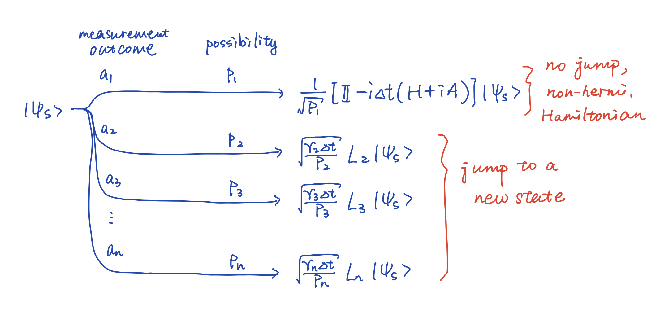is conditioned on the measurement outcome. Namely, starting from a pure states , two distinct types of operations were possible:

Here $p1 = 1-\Delta t \sum{\alpha >1} \gamma\alpha \langle \psi_s|L\alpha^\dagger L\alpha | \psi_s \ranglep\alpha = \gamma\alpha \Delta t \langle \psi_s|L\alpha^\dagger L_\alpha | \psi_s \rangle$. The possibilities are the overlap between the state before and after the jump.

Consider this as a PDP, we have:

• between the jumps the state evolves by a non-Hermitian: $\psi(t+dt) = \frac{1}{\sqrt{p_1}}(\mathbb{I} - idt[H+iA])\psi(t)\tag{3.6}$ note that we can write $p1 = 1-xx \sim dt\frac{1}{\sqrt{p_1}} = \frac{1}{\sqrt{1-x}} \approx 1+\frac{1}{2}x = 1+\frac{1}{2}dt \sum{\alpha >1} \gamma\alpha |L\alpha \psi|^2$.
• jumps occur with probabilities $p{\alpha>1}$\psi(t+dt) = \sum{\alpha>1} (\frac{L\alpha \psi}{|L\alpha \psi|}-\psi) dN_\alpha\tag{3.7}$$

In total, we get:

$$\begin{aligned} d\psi(t) &= \psi(t+dt) - \psi(t)\\ &=-i(H+iA)\psi(t)dt + \frac{1}{2}\sum_{\alpha>1}\gamma_\alpha \|L_\alpha \psi\|^2 \psi(t)dt +\sum_{\alpha>1} (\frac{L_\alpha \psi}{\|L_\alpha \psi\|}-\psi) dN_\alpha(t) \end{aligned}\tag{3.8}$$

3.3 Connection between quantum trajectories and the density matrix

The projection of the enviornment measurement divide the Hilbert space into subspaces. The probability for a subspace can be expressed in the functional of density :

$$\mu(A) = \int_A \mathcal{D}\psi \mathcal{D}\psi^* P[\psi]\tag{3.9}$$

For any functional , we can use the distribution to compute the expectation value:

$$E(F[\psi]) = \int \mathcal{D}\psi \mathcal{D}\psi^* P[\psi]F[\psi]\tag{3.10}$$

• The expectation value of an observable : .
• The density matrix: . .